Fourier Series and Laplace Transform the cornerstone of control theory and signal processing: Turning complexity into clarity.

---What we know is not much. What we do not know is immense.
(Pierre-Simon Laplace)

---According to Fourier Series, everything is linked together in a sinusoidal, nonlinear pattern, events will always repeat itself

---According to Fourier Transform, you can break down complex task into array of simple tasks and repeat it as a periodic function .

▶ Watch the video, Fourier and Laplace
▶ Watch the video, digital signal

Fourier Series and Laplace Transforms turn complex time-based differential equations into simple algebra, creating clarity for control theory and signal processing

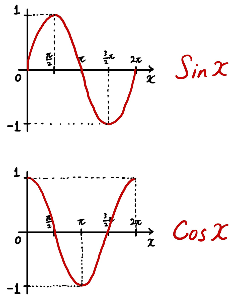
Jean-Baptiste Joseph Fourier was a French mathematician and physicist , he gave us the mathematical expression of an event that repeat itself in a sinusoidal, non linear pattern,

While Pierre-Simon, Marquis de Laplace, a French national, gave us an insight into how time domain function of a sinusoidal system (frequency )can be derived.

Both French nationals helped us to shape our understanding of a control system and signal conditioning.
A complex task or signals can be broken down into a simple discreet or arrays.

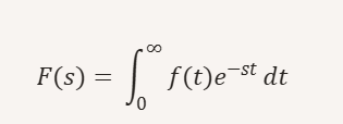
Fourier Series and Laplace Transform are two cornerstone mathematical tools: Fourier Series decomposes periodic functions into sums of sines and cosines (frequency components), while the Laplace Transform converts time-domain functions into algebraic expressions in the complex frequency domain, making differential equations easier to solve.

Fourier Series

Definition: Represents a periodic function as an infinite sum of sine and cosine terms.
Formula (for period 2L):

where coefficients are computed by integrating the function against sine/cosine basis functions.

Applications:
- Signal processing (breaking down audio or electrical signals into harmonics).
- Solving partial differential equations (e.g., heat equation).
- Engineering problems involving vibrations and waveforms.
Key Notes:
- Works only for periodic functions.
- Convergence depends on function smoothness (Dirichlet conditions).
- Discontinuities cause the Gibbs phenomenon (overshoot near jumps).
Laplace Transform
- Definition: Converts a time-domain function f(t) into a complex frequency-domain function F(s).
- Formula:
Laplace time domain

where s is a complex variable.
- Applications:
  - Solving linear differential equations by turning them into algebraic equations.
- - Widely used in control systems, circuit analysis, and mechanical systems.
- - Handles initial conditions naturally, unlike Fourier series.
- Key Notes:
  - Useful for non-periodic functions.
- - Related to the Fourier Transform but more general (includes exponential decay factor for convergence).
- - Inverse Laplace Transform retrieves the original time-domain function.
- control theory

Practical Insight

Fourier Series is best when analyzing periodic signals (e.g., sound waves, alternating current).
Laplace Transform is best when solving differential equations with initial conditions (e.g., electrical circuits, mechanical systems).
Together, they form the backbone of engineering mathematics, especially in signal processing, control theory, and physics.

breaking a problem down into simple, discrete steps is the most effective way to tackle complexity. It’s the same principle behind algorithms, project management, and even mathematical tools like the Fourier Series and Laplace Transform we discussed earlier: each takes a big, messy problem and reduces it into manageable parts.

Here’s a quick framework you can apply to almost any situation:

🧩 Step-by-Step Problem-Solving

Define the problem clearly
- What exactly needs to be solved?
- Avoid vague statements; be precise.
Break it into smaller chunks
- Divide into sub-problems or stages.
- Each chunk should be solvable on its own.
Prioritize the order
- Which step must be solved first?
- Some parts depend on others, so sequence matters.
Solve each piece independently
- Focus on one discrete unit at a time.
- This reduces overwhelm and increases accuracy.
Integrate the solutions
- Combine the solved parts into the whole.
- Check if they fit together smoothly.
Test and refine
- Verify the complete solution works.
- Adjust if any piece doesn’t align.

⚡ Example: Solving a Differential Equation

Big problem: Solve y′′+3y′+2y=0.
Breakdown:
1. Identify it as a linear ODE.
2. Write characteristic equation: r2+3r+2=0.
3. Solve roots: r=−1,−2.
4. Build solution: y(t)=C1e−t+C2e−2t.
Each step is simple, but together they solve the whole.

This approach works whether you’re debugging code, planning a project, or even learning a new concept. It’s essentially the art of decomposition — turning complexity into clarity.

How They Work

Time Domain vs. Transformed Domain: Real-world signals change over time and involve calculus (derivatives and integrals) through circuit components like capacitors. Transforms move these signals into a frequency or exponential domain where math becomes basic algebra.

Fourier Series: Breaks any periodic signal down into a simple sum of sine and cosine waves (or complex exponentials).

Fourier Transform: Extends this idea to non-periodic signals to analyze the entire frequency spectrum.

Laplace Transform: Generalizes the Fourier transform by adding a damping factor .This allows analysis of unstable or growing systems where standard Fourier transforms fail

Core Applications

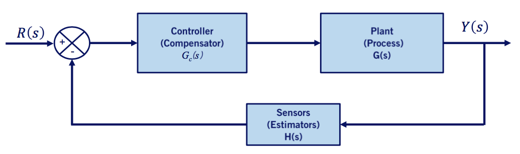
Control Systems: The Laplace transform creates a system transfer function (output divided by input), letting engineers analyze stability using poles and zeros on the s-plane.

Signal Processing: Fourier methods decompose signals into specific frequencies for filtering, communication, and spectral analysis

Fourier Series and Laplace Transform the cornerstone of control theory and signal processing: Turning complexity into clarity.

Comments (0)